Using Weibull Analysis to Plan Maintenance
Weibull analysis can be used to examine a myriad of failures and problems, including equipment breakdowns. By better understanding why and when breakdowns happen, companies can better tailor their maintenance programs to limit downtime and improve productivity.
Here are three scenarios in which Weibull analysis improves maintenance programs.
Preventive Maintenance
The first example involves a fleet of 34 trucks, seven of which failed while on the job. Technicians determined the failure was due to a component in the fuel subsystem that made the engine stall without warning and prevented drivers from restarting the engine. These failures created safety concerns and were expensive to repair because trucks had to be fixed while out on the road.
Most trucks in the fleet had not had a failure, so the Maximum Likelihood Estimation (MLE) technique was chosen to perform a 2-parameter Weibull analysis. MLE analysis is preferred over the alternative, the Ranked Regression technique, when the data contains a large number of non-failed (suspension) data.
Related
Weibull Plots Predict System Reliability
Calculating Machine Reliability from Bearing Life
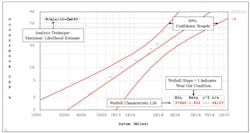
A close inspection of the results (Analysis for Truck Problem) indicates the data is well represented by a two-parameter Weibull distribution. The failure data points align with the predicted result and fall well inside the two-sided 90% confidence bounds used in this analysis. Note that only failure data is plotted when using MLE or RR techniques.
The two parameters of interest in the analysis are the characteristic life (Eta = 37,680 miles) and slope of the Weibull line (Beta = 1.552). In the analysis, the fuel subsystem component was showing a slight wear-out condition, based on the fact that the value of Beta is greater than 1. This would lead to an optimal time of replacement analysis based on the total cost of maintenance.
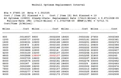
Although maintenance costs for component replacement in the shop were well known, maintenance costs for repairs on the road needed to be calculated. These included the mechanic’s travel costs, maintenance vehicle costs, downtime for the disabled truck, including the cost for the stranded driver, and the cost of lost reputation due to late deliveries. The cost analysis showed that failures cost 10 times that of a scheduled replacement. Using this 10:1 ratio, the company performed an optimal time of replacement analysis (results shown inTable 1).
As can be seen from the table, the best time to replace the component and minimize costs is at 13,800 miles. If fleet reliability were more important than cost, however, the same analysis results can determine the best time for replacement based on the need to keep the fleet up and running.
Early Failures
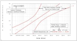
In this example, a transport company began having failures of a component in their buses’ fuel subsystems and requested an analysis of their limited dataset. There were a total of 31 buses in the fleet and four recent failures were of great concern because they led to emergency repairs. The buses were not new, but the failures were, so it took some thought in developing the dataset for analysis. After discussions with maintenance personnel, the dataset was based on the last time the component of interest was replaced (results shown in Analysis for Bus Problem).
As with the previous example, MLE analysis was chosen based on the high number of non-failed components. The results show a wide 90% confidence bound around the data. This is due to the low number of failures. Failures seem to align well with the predicted Weibull analysis plot, leading to the conclusion that the dataset conforms to a two-parameter Weibull distribution. The characteristic life, Eta=319,742 miles, is also quite large and implies that the “failing” component is quite robust and should not be failing that often. This can be put into perspective by calculating the mean miles between failure (MMBF) using the following equation:
MMBF = Eta*Γ(1 + 1/Beta)
MMBF = 319742* Γ(1+1/0.613) = 468247 miles
This means the average component should not fail during the lifetime of a bus. As mentioned previously, the Beta value is critical to good maintenance decisions. In the current example, Beta is much less than 1, indicating the failures are an extreme case of infant mortality (premature failure). Although infant mortality is common in electronic equipment, which often requires environmental stress screening to weed out weak parts prior to shipping them, it is far less common in mechanical components. A long-term solution to this problem requires more information.
After some hunting for the right information, it was discovered that the failing component, a brass elbow, was replaced when another component was serviced because it was convenient, and that the elbow was failing due to clogging. This should not have happened as there was a pre-filter just before the elbow.
A decision was made to replace the pre-filters and elbow when maintenance was performed. This was a case when unusual data led to the usual questions to the right people and a solution was found.
This example highlights several aspects of a maintenance analysis:
• Throwing more maintenance at a problem is not necessarily a solution.
• Everyone’s input is important in identifying the problem and potential solutions.
• Act on what the data is telling you, especially the value of Beta according to the Weibull analysis.
Constant Failure Rate
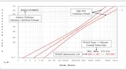
This scenario involves a two-parameter Weibull analysis of a line replicable unit (LRU) on a helicopter. The LRU was not a flight-critical component, so the goal of the analysis was to determine the best replacement interval (results shown in Analysis for Aircraft Problem). By definition, LRUs are not repairable when they are replaced and they often fail due to several causes. As a result, the Weibull plot may show competing failure modes. The other possibility is that a large number of competing failure modes may blend together in the analysis, making it impossible to separate failure modes without more effort and information.
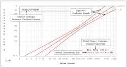
As with the previous examples, MLE was used to perform a two-parameter Weibull analysis. Results show a good correlation between plotted failures and the analysis’ prediction. The high number of failures also yields much tighter confidence bounds. The fact that all plotted failures fall inside the 90% confidence limits is another indication of a good fit to the data.
Related
Weibull Plots Predict System Reliability
Calculating Machine Reliability from Bearing Life
The characteristic life, Eta=3,423 hours, was much higher than the customer’s expectations, which helped with the “bad news” about Beta. A Beta value of approximately 1 indicates that LRUs were failing at a constant failure rate. This could be due to a single failure mode or a mix of a large number of failure modes, but separating the data was unlikely with the information available.
A constant failure rate is problematic from a maintenance perspective. As the failure rate does not change with age, newly installed components have the same probability of failing in the next hundred hours of operation as ones that have been running for 1,000 hours. In such cases, proactive maintenance does you no good. This leads to two alternatives; redesign the component if it’s not meeting its reliability requirement, or run the component to failure before replacing it. Fortunately, the LRUs were exceeding their reliability requirement.
These three examples show how Weibull analysis can guide maintenance strategies. Understanding a component’s underlying failure distribution is critical in determining whether preventive maintenance is appropriate, and, if so, at what interval. It’s equally important in understanding preventive and corrective maintenance intervals, preventive and corrective replacement costs, and equipment design life. Finally, a clear understanding of safety and mission reliability requirements is critical for improving preventive maintenance programs.
Paul Lein is Senior Engineer and David Nicholls is Director of RMQ Engineering at Quanterion Solutions Inc. in Utica, N.Y.
