Unlocking Weibull analysis

|
Authored by:
|
When products start failing, management wants answers. Are they failing because of manufacturing problems? Or is the design to blame?
One of the most widely regarded methods for ferreting out the reason behind failures, as well as accurately predicting operational life, warranty claims and other product qualities is statistical analysis of a component’s or device’s failure data. Though there are many statistical distributions that could be used, including the exponential and lognormal, the Weibull distribution is particularly useful because it can characterize a wide range of data trends, including increasing, constant, and decreasing failure rates, a task its counterparts cannot handle. This characteristic also lets Weibull distributions mimic other statistical distributions, which is why it is often an engineer’s first approximation for analyzing failure data.
What Weibull analysis can do
Many management decisions involving life-cycle costs and maintenance can be made more confidently from reliability estimates generated by Weibull analysis. For example, Weibull analysis can reveal the point at which a specific percentage of a population (such as a production run) will have failed, a valuable parameter for estimating when specific items should be serviced or replaced. Additionally, this analysis helps determine warranty periods that prevent excessive replacement costs as well as customer dissatisfaction.
Weibull analysis can be particularly helpful in diagnosing the root cause of specific design failures, such as unanticipated or premature failures. Anomalies in Weibull plots are highlighted when items uncharacteristically fail compared to the rest of the population. Engineers can then look for unusual circumstances that will help uncover the cause of these failures, which could include a bad production run, poor maintenance practices, or unique operating conditions, even when the design is good.
In addition to these factors, understanding the time and rate at which items fail contributes to other reliability analyses such as:
▶ Failure modes, effects, and criticality analysis
▶ Fault tree analysis
▶ Reliability growth testing
▶ Reliability centered maintenance
▶ Spares analysis
As with most analytical methods, the accuracy of a Weibull analysis depends on the quality of the data. For valid Weibull analysis, and to interpret the results, there are several requirements for the data:
▶ It must include item-specific failure data (times-to-failure) for the population being analyzed.
▶ Data for all items that did not fail must also be included.
▶ The analyst must know all experienced failure-mode root causes and be able to segregate them.
Engineers often shy away from Weibull analysis because they believe it is too complex and esoteric. Although it’s true that an understanding of statistics is helpful, engineers can reap the benefits of a Weibull analysis without a strong statistical background.
The Weibull distribution generally provides a good fit to data when the quality of that data is understood. Values for the resulting distribution parameters help explain an item’s failure characteristics. These qualities can then influence cost-saving decisions made during design, development, and customer use. And when the distribution does not provide an acceptable fit, the qualities of the Weibull plot may still point the way to alternative distributions that might provide a better fit.
Weibull terminology
Here are important terms in a two-parameter Weibull analysis:
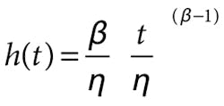
Hazard Rate:
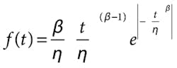
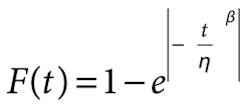
Cumulative Density Function (CDF):
Data types
The accuracy of any analysis depends on the type, quantity, and quality of data being analyzed. There are two categories of data used in a Weibull analysis: time-to-failure (TTF) and censored (or suspension) data.
As the name implies, TTF data indicates how long an item lasts before failing. It can be measured in hours, miles, or any other unit that defines a product’s life. In some cases, the life of different parts of an item may be described by different metrics. For example, on airplanes, engine failures can be reported based on flight hours, while landing gear failures are tracked by the number of landing cycles. Failures in different parts of an item must be treated separately for analysis and then combined to create a system-level life prediction. TTF data should also be associated with a specific failure mode for the part whenever possible. This data can come from various sources, including reliability growth testing, reliability qualification testing, and maintenance databases of field data.
Censored data represents failure data recorded over an operating or test period. It can be broken down into three categories, Right-censored data includes test/operating times for items that did not fail (suspensions) and those that did. Interval data includes all failures within a specific time interval, but the exact time-to-failure is unknown (e.g., warranty data). For left-censored data, the exact time an item failed is unknown, other than the failure occurred before it was discovered.
Although Weibull analysis can be done without considering individual root failure causes, knowing and segregating failure modes lets engineers extract information about the item’s reliability.
A decreasing failure rate (infant mortality or product failing soon after being made) is generally attributed to problems with manufacturing or part quality. It indicates that reliability of the remaining products soon improves as defective items fail quickly and are weeded out. The rest of the items, considered defect free, either fail at a relatively constant rate or at an increasing rate as they wear out. Constant failure rates are common for electronic devices and complex systems due to the large number of different possible failures. Most mechanical item failures, however, are caused by wearout.
Performing Weibull analysis
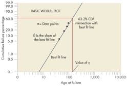
The traditional approach to performing two-parameter Weibull analysis is by plotting the data (usually done using commercial software). Each failure time is ranked based on the number of items that did and did not fail at that time, with the most popular rankings being mean and median. The data is then plotted manually or by software on Weibull probability “paper,” .
Commercial software like WinSmith, SuperSMith, or Quanterion’s QuART-ER, simplifies analysis by automatically ranking and plotting failure data. Tools vary widely in price and can typically be downloaded off the internet.
A best-fit line drawn through the data points lets engineers determine how well the underlying statistical distribution fits the data. If the fit is valid, the best-fit line provides the item’s characteristic life and failure rate over time. If the distribution does not provide an acceptable fit, the Weibull plot’s qualities can identify a more appropriate distribution or suggest a better interpretation of the data. For example, there may be other failure modes, a sudden change in the predominant cause of failures, or items were used in different environments. Plot features such “knees” (corners) or S-Shapes often indicate one or more of these problems may be responsible.
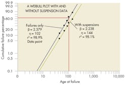
It is critical to understand that even though right-censored data is not plotted as part of a Weibull analysis, it significantly affects rankings that determine the Weibull plot’s shape. Omitting data on items that don’t fail can generate results that underestimate an item’s true reliability. (See A Weibull plot using data with and without suspension.) This can prove costly in terms of more maintenance actions, inventory of spares, and an unnecessary redesign to improve reliability. Analysts should include all pertinent data to ensure accurate analysis results and interpretations.
Assessing the fit
Regardless of the technique used, an analyst must assess the assumed statistical distribution’s fit to a dataset. The failure data plot is particularly useful, as it not only allows for a simple check of whether a linear fit matches the data, but can also indicate potential solutions when the fit is not linear.
Other statistical tests that quantify the goodness-of-fit to particular distributions include the Chi-square, Kolmogorov-Smirnov, and Anderson-Darling tests. Each has advantages and disadvantages, depending on the quantity of available data and the distribution being analyzed. Information on these tests can be found in most reliability and statistics books.
To this point, a good linear fit to a dataset has depended on selecting an appropriate statistical distribution. However, this can be complicated.
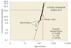
Consider a case in which the failure data were recorded for a single failure mode of a mechanical component that led to a device failure. (See A poor 2-parameter Weibull plot.) The failures occurred in a long-term storage environment and were not discovered until the devices were removed for periodic testing. This particular failure mode was deemed critical due to the large number of failures. Despite the fact most devices worked when removed for periodic testing, suspensions (those that passed the testing) were not recorded in the original dataset. This dataset, then, could not be used to estimate the population’s reliability. Data from this testing can still be used, however, to illustrate different filtering techniques that can improve a distribution’s fit to a dataset.
Because the devices were in storage, failures were not discovered until they were tested. Actual failure times are unknown, so interval (failure discovery) data must be used for analysis. There are also distinctive “knees” in the plotted results, which can indicate several different types of failures, different operating environments, poorly manufactured lots, or parts made by different manufacturers. In this example, the reason for failures was known, storage environments were similar, and all parts were made by the same manufacturer. Consequently, further investigation was needed to identify the reason for the discrepancies.
A review of serial numbers of failed parts did not reveal any indications of a manufacturing issue. However, it did indicate that failed parts were from two different versions of the device. Although the mechanical part was identical in both designs, data was filtered by version and an independent analysis performed on the two datasets.
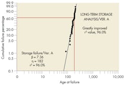
Plotting “Version A” data shows a noticeable improvement in the linear fit to the plot. The high beta value, 7.36, suggests a rapid wearout condition for the failing parts in this version.
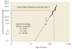
A Weibull plot for “Version B” data (Figure 7) has a best-fit line with a smaller beta (3.02). Though used in two different versions of the same device, the actual part, reason for failure, and storage environment were identical, so there should not be a sizeable difference between beta values for these two datasets.
It was subsequently determined that the difference between the two versions was the test circuitry used to diagnose mechanical-part failures. Thus, failure data for the two designs were based on two different test units. Analysts questioned whether the mechanical part or test circuitry was responsible for the failures.
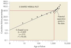
Another problem arises when the Weibull plot creates an S-shaped profile around the best-fit line. It usually means a mixed dataset (See S-shaped Weibull plot). Standard filtering techniques can separate the datasets to get accurate results. This requires identifying the reason why there are different failures in the dataset. It could be:
▶ More than one reason for the failures.
▶ The same reason for failure, but different operating environments.
▶ The same reason for failure, but different part manufacturers or production lines.
▶ Closely grouped set of serial numbers (indicating a bad production lot).
▶ Same type of failures but different reasons.
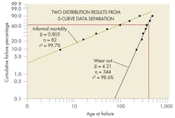
If you can’t find the reason, you can still try to categorize failures through statistical means. One approach is to assume the datasets are “appended” together with no overlap in failure times. You can test each potential separation point around the main inflection point looking for the best statistical result. The statistical test is based on the goodness-of-fit for the two resulting distributions (See Two distribution results from S-curve data separation).
The goal of a Weibull analysis is to estimate the reliability of an item in a specific application or environment. Results are used to estimate reliability and the adequacy of a design, and for developing maintenance schedules and inventories of spares.
Using statistical analysis, it is easy to predict reliability. Since the y-axis coordinates on the Weibull plot refer to the percentage values of the CDF, the reliability can be determined directly from the plotted dataset.
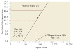
Once the Weibull parameter values are known, reliability estimates can be calculated using the Weibull reliability function, R(t). The reliability function can also be mathematically manipulated to solve for a reliability/life prediction for an item population. For example, one could calculate a B10 life, which is equivalent to the time when the population’s reliability is 90%. (See Predicting B10 Life.)
Reliability predictions can also be performed on separated datasets, such as those for an item with competing failure modes, operated in different environments, produced by different manufacturers, etc. The prediction requires the use of a scaling function to address the impact of each failure mode distribution on the overall item’s reliability.
Resources
▶ The New Weibull Handbook – Fifth Edition, Gulf Publishing Co., 2007, by Abernethy, Dr. R.B., (http://tinyurl.com/cdrypo9)
▶ Applied Life Data Analysis, John Wiley & Sons, 1982, ISBN 0471094587, by Nelson, W. (http://tinyurl.com/cz4cl39)
▶ Mechanical Analysis and Other Specialized Techniques for Enhancing Reliability – MASTER, Reliability Information Analysis Center, 2012, ISBN 978-1-933904-39-9, by Rose, D., MacDiarmid, A., Lein, P., et al (http://tinyurl.com/cqlyt7f)
About the Author
Voice Your Opinion!
To join the conversation, and become an exclusive member of Machine Design, create an account today!

Leaders relevant to this article: