
Programming quantum computers is vastly different than programming conventional ones. To get a better idea of what it could be like, this article steps through the process of programming a quantum computer, a D Wave System Two, using the direct embedded method to solve a relatively simple problem.
Glossary |
|
Coupler: A variable (b) that defines how two qubits Qubit: A variable (q) that has a value from the set {0, 1}. Quantum Machine Instruction (QMI):A restatement of the problem to be solved. The computer comes up with a distribution of qubit values that minimize the value of the QMI. Strength: Defines the coupler relationship between qubits and provides another way to influence qubits. A coupler connecting qubits qi and qj has a strength of b and is denoted bij. Weight: In the QMI, each qubit (q) is given a weight (a) as one way of influencing qubits. For example, qubit, qi has a weight of ai. |
The problem
Map coloring is a type of combinatorial optimization problem. For this problem, the goal is to color the 13 territories and provinces of Canada so that no two regions sharing a border are the same color, and regions touching only at one or more isolated points, such as Nunavit and Saskatchewan, are not considered to share borders. There are also a limited number of colors, C.

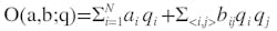
The programming involves variables defined in the glossary and the objective function described in the previous article (Quantum Computing 101):
Next, choose a correspondence or encoding between colors for a region and the qubit values. After fixing the encoding, work out the form of a quantum machine instruction (QMI) that will give valid colorings. This task is broken into four steps:
1. Turn on one of several qubits.
2. Map a single region to a unit cell.
3. Implement constraints using couplers.
4. Clone neighbors to meet similar constraints.
Using unary encoding for the possible colors for each region, assign C qubits to each region of the map. If the ith color is assigned to a region, then the ith qubit (qi) associated with that region will have the value 1 in our samples (or results from the quantum computer) and the other (C – 1) qubits associated with that region will have the value 0.
This file type includes high resolution graphics and schematics when applicable.
Turn on one of C qubits
First, solve the simpler problem of turning on just one qubit in a two-qubit system. For a two-qubit system, the objective becomes:
O(a, b; q) = a1q1+ a2q2+ b12q1q2
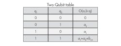
The four possible states in the distribution are listed in the Two-Qubit System Table. Choose a1, a2and b12 values so that the distribution consists of the states with q1= 0 and q2= 1 and the one in which q1= 1 and q2= 0. The other two states in which qi’s equal 0 or 1 should not be in the distribution.
To make encodings of either color equally likely in the distribution, a1 must equal a2. These values also need to be less than 0 so that the state characterized by q1= 0 and q2= 0 will not appear. Therefore:
a1 = a2 < 0
To eliminate the state in which q1and q2 equal 1 from the distribution requires that:
a1+ a2+ b12 = 0
A solution to these equations is:
a1= −1, a2= −1, and b12= 2
Substituting those values for a1, a2and b12into the Two-Qubit System Table shows that the objective value is minimized for the two states in which one qivalue is 1 and the other is 0. This means samples from the distribution generated by the QMI will consist solely of these two states.
These coefficient values would be enough if the map had only two colors, but most maps require more colors. Therefore we must generalize to the case where C qubits represent the possible colors assigned to a region. The goal is to find values of aiand bijcoefficients that will yield a distribution over those samples that have exactly one qubit turned on (equal to 1) and the other C − 1 qubits turned off (equal to 0).
To solve this problem, take a clue from the two-qubit problem. In that problem, two states needed exactly one qubit turned on to be equally represented in the distribution and thus we set a1= a2. The solution is symmetric if the two qubits are interchanged, as expected.
Now apply this principle to the case with three colors, along with a corresponding number of qubits to simplify the constraints.
If C = 3, then there are three qubits. The corresponding objective function is:
O(a, b ; q) = a1q1+ a2q2+ a3q3+ b12q1q2+ b13q1q3+ b23q2q3
Simplify this objective by applying the insight about the symmetry of the solutions, and require the three aivalues equal one common value, a. Similarly, require the three bijvalues equal a common value b:
O(a, b ; q) = a(q1 + q2+ q3) + b(q1q2+ q1q3+ q2q3)
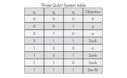
Tabulate the eight states of this system (see the Three-Qubit System Table).
Taking a hint from our previous example, observe that setting a = −1 and b = 2 will give the three states with exactly one qubit turned on an objective value of −1. Among the other five states, four will have objective values equal to 0 and one will have its objective equal to 3. This guarantees samples will consist only of qubit patterns with one of the three qubits is equal to 1.
A quick check confirms that this same symmetry argument can be applied to problems with C = 4 or higher. In all these cases, the distribution is influenced to contain only qubit patterns with exactly one qubit turned on by choosing ai= −1 for all the weights and bij= 2 for all the strengths.
Map a single region to a unit cell

To finish the first step of transforming the map-coloring problem to a QMI, C qubits were introduced for each region in the map and weights and strengths for the qubits and couplers were initialized. The connectivity pattern of the qubits and couplers is represented in the figure Connectivity of Qubits and Couplers. It illustrates how each graph vertex represents a qubit and each edge represents a coupler between qubits. The Unit Cell figure depicts a small portion of the pattern of physical qubits and couplers corresponding to the unit cell. It is easy to find many instances of the complete graph on two vertices, but there are no instances of the complete graph on three or four (or more) vertices. This poses the next challenge.
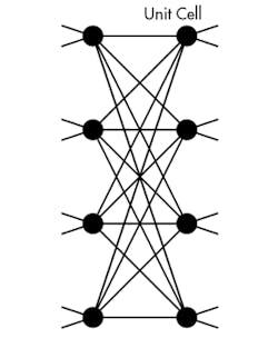
To solve this problem, make a distinction between logical qubits and couplers and physical qubits and couplers inside the quantum computer. Each logical qubit corresponds (via an embedding) to one or more connected physical qubits, which is called a chain. To implement a coupler between logical qubits, it is enough to find a physical coupler connecting any physical qubit in the chain for the first logical qubit to another physical qubit in the chain for the second logical qubit.
This strategy makes it easy to map complete graphs on up to four vertices to the unit cell in the computer. The chain for the first logical qubit corresponds to the top two physical qubits in the unit cell. Likewise, the chain for the nth logical qubit corresponds to the two physical qubits in the nth row of the unit cell. It is easy to confirm there is a physical coupler between each pair of chains, yielding a unit-cell embedding for complete graphs of up to four vertices.
To ensure the physical qubits within one chain faithfully represent a single logical qubit, we must define weights and strengths for the physical qubits within a chain that keeps them aligned.
By referring to the table of objective values for the two-qubit system, it is easy to see that assigning a1= 1, a2= 1, and b12= −2 give the aligned chains an objective of 0 and misaligned chains an objective of 1. Note that the weight and strengths necessary to implement this desired set of states are negative versions of the weights and strengths used to solve the “1 of 2” problem.
To complete this step, supply a rule to map weights and strengths for logical qubits and couplers to the physical qubits and couplers that represent them. Each logical qubit is represented by a chain of length two so we divide the weight of -1 for the logical qubit in half and apply a weight of -1/2 to each physical qubit in the chain.
Likewise, we specified a strength of 2 for logical couplers. Because the chains for each pair of logical qubits are connected by two physical couplers, we also divide the logical strength of 2 into two physical strengths of 1 each in the unit cell.
Implement constraints using couplers
At this point, colors are encoded for each region using logical qubits, and the logical qubits and couplers are mapped to physical unit cells. Now we need to enforce the neighbor constraints. With some foresight, we chose the unary encoding and logical-to-physical mapping to simplify this next step (and the following one, too).
The task is to adjust the weights and strengths so that when, for example, the red qubits for British Columbia and Alberta both turn on, it increases the value of the objective function. On the other hand, the objective should stay constant when both these red qubits are turned off or when one or the other (but not both) is turned on.
Referring to the Two-Qubit System Table, assume q1 refers to British Columbia’s red qubit and q2refers to Alberta’s red qubit. By setting a1= 0 and a2= 0 and b12= 1, the objective is lifted in the fourth state, which we need to penalize, and leaves the other three states at an objective of 0.
To implement this penalty, it will take a physical coupler that connects British Columbia’s and Alberta’s red qubits. This requires a look at a slightly larger portion of the fabric of physical qubits and couplers that make up the D-Wave computer.
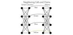
The figure Neighboring cells and chains shows two neighboring unit cells and highlights the chains in each unit cell that represent the four logical qubits, one for each color. Most importantly, for the current step, this figure also represents physical couplers connecting two adjacent unit cells as arcs.
It is clear these couplers are ideally positioned to implement the portion of the objective that ensures that if the chain representing color i is turned on in one unit cell and the chain representing color i in the neighboring unit cell is also turned on, it will penalize this state. So the strength associated with the four arc-shaped couplers should be set to 1.
Clone regions as necessary
This last step in mapping the coloring problem to the quantum-programming model is necessitated by neighbor relations in the map and connectivity of unit cells. To appreciate this problem, note that British Columbia, Alberta, and the Northwest Territories are all neighbors. Also note that unit cells are configured in a two-dimensional checkerboard array. The configuration of these three regions cannot be mapped to unit cells while preserving the neighbor relation.
We could assign British Columbia and Alberta to unit cells that neighbor each other horizontally (see Neighboring cells and chains) and assign the Northwest Territories to a unit cell positioned vertically above British Columbia. This configuration means Alberta is not a direct neighbor of the Northwest Territory in the unit-cell array and, hence, no physical couplers are available to ensure the same color qubits will not be simultaneously activated in these two regions.
Using clones can solve this problem, though. Clones are analogous to chains of physical qubits representing a single logical qubit. In this case, several unit cells represent the color of a single region. Just as with chains of physical qubits, cloning extends the footprint of a single region in the unit-cell array to provide more neighbors for a cloned region. This lets us enforce neighbor constraints arising from Canada’s map that do not transfer directly to the unit-cell array.
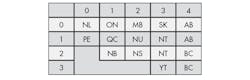
The Map of Canada in Unit Cell Array maps Canada’s 13 regions to unit cells with Alberta (AB), British Columbia (BC), and the Northwest Territories (NT) all cloned. It is easily checked by referencing the Map of Canada that each neighbor relation from the map of Canada corresponds to some adjacent pair of unit cells in the cell array.
To complete this step, the strengths for the intercell couplers must be adjusted so that the color assigned to Alberta in the unit cell in row 0 and column 4 matches the color assigned to Alberta in the unit cell in row 1 and column 4. This problem is solved in exactly the same way as solving for chains of physical qubits representing a logical qubit. For the physical coupler connecting the red qubits in Alberta’s top and bottom cells, adjust the strength of the coupler to -2 and add a weight of 1 to the two physical qubits connected through the coupler. Repeat this for each of the other colors as well as for British Columbia and Northwest Territories, which have also been cloned.
These four steps transformed the problem of generating a valid coloring for the regions of Canada into a single QMI for a quantum computer. They followed naturally from the decision to represent colorings via a unary encoding scheme, which requires 13C qubits to represent the possible C colorings of the 13 regions of Canada. (Implementing the steps in a conventional programming language such as C is shown in an appendix available to those who request it via email to mdeditor with quantum n the subject line.)
Regardless of language, standard constructs generate the weights and strengths of the QMI. Special library routines are used to pass the QMI to the D-Wave computer and retrieve samples from the resulting distribution.
Three conclusions can be drawn immediately from this exercise. First, mapping this problem to a QMI could be simplified via routines which create embeddings of a logical formulation to a physical QMI. Second, the size of a map that can be colored using this strategy is limited by the number of unit cells available in the computer. A more scalable strategy would include the ability to divide larger maps into chunks that can be handled individually. Results from several chunks could be synthesized to create the coloring of larger maps. Finally, the D- Wave unit cell is large enough to handle four colors with this encoding, but the scheme needs to be modified to handle more general mapping problems that use more than four colors.
This file type includes high resolution graphics and schematics when applicable.
About the Author
E. D. Dahl
Senior Research Scientist
Voice Your Opinion!
To join the conversation, and become an exclusive member of Machine Design, create an account today!

Leaders relevant to this article: