Design Essentials: S-Curves and Linear Motor Sizing

Download the PDF of this article.

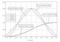
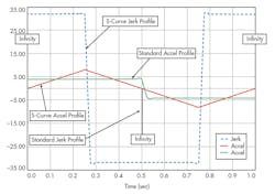
In high-throughput applications, standard triangular or trapezoidal motion profiles have been widely utilized to reach a desired position quickly. As shown in the velocity and position profile image, triangular velocity profile consists of a period of constant acceleration to a maximum velocity, followed by a period of constant deceleration back to zero. With the standard triangular profile the acceleration increases or decreases almost instantaneously, as shown in the acceleration and jerk profile graph at time 0.0, 0.5, and 1.0.

In these locations, the rate of acceleration change (da/dt) is undefined and equal to infinity. The rate of acceleration change is given the name Jerk, j = da/dt. In high-throughput applications, the undefined jerk will cause impact loading, residual vibration, and possibly audible noise. Introducing S-Curves or 2^nd order polynomials in the velocity profile, as shown in velocity and position profile, allows the Jerk to be finite and the motion to be smooth.

These S-Curves are programmed in the motion controller and not limited to a specific drive technology. However, this article will focus on S-curves and linear motors sizing in particular, since linear motors are used in the most demanding of point-to-point applications.

Profiles

The first step in sizing a linear motor with S-Curves is to determine the motion profile parameters such as maximum velocity (v_max), maximum acceleration (a_max), and RMS acceleration (a_RMS), given the total move distance (s_t), total move time (t_m), and duty cycle or dwell time (d_w). For example, the application may call for a point-to-point motion of 1.0 meter in 1.0 second with an 80% duty cycle or dwell time of 0.25 seconds.

To calculate the motion parameters we will first assume a triangular profile with full S-Curve and then apply, if known, any maximum speed or acceleration constraints. The constraints in maximum velocity may be due to the linear bearings, linear encoder, limited controller data rates, or available supply voltage. The constraints in maximum acceleration may be due to the linear bearings, amplifier peak current, or structural stiffness.

If there is a speed constraint, the motion parameters can be calculated using the 1/3 trapezoidal or general trapezoidal motion profiles with full S-Curve, which have lower speed but higher acceleration requirements than the triangular motion profile. With an acceleration constraint, the total move time (t_m) may have to be increased, since the triangular motion profile already has the lowest acceleration requirements.

Machinedesign Com Sites Machinedesign com Files Uploads 2017 03 30 0517 Md Motor Sizing Velocity Distance Profiles

The graph above depicts velocity and position profiles for linear motors.

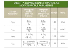
The maximum velocity (v_max), maximum acceleration (a_max), and RMS acceleration (a_RMS) can be calculated for the example of 1 meter in 1 second, using the formulas for the triangular profile with full S-Curve in Table 1. The maximum velocity is calculated to be 2.0m/sec with a maximum acceleration of 8.0m/sec² and a RMS acceleration of 4.62m/sec². It is important to recognize the penalty for using the full S-Curve velocity profile compared to the standard velocity profile, given the same total move distance (s_t) and total move time (t_m).

While the maximum velocity is the same for both motion profiles, the maximum acceleration is 2× greater in the triangular profile with full S-curve. The maximum acceleration of the full S-Curve profile occurs at time 0.25 seconds, which is the midpoint of the acceleration period. The second penalty for using the full S-Curve velocity profile over a standard velocity profile is a 33% increase in the continuous power dissipated by the linear motor. In Table 1 the continuous power is shown by the parameter P_RMS, which is also expressed by the following formula (1.1):

Machinedesign Com Sites Machinedesign com Files Uploads 2017 03 30 Equation A

In the above formula, F_RMS is the continuous force applied by the linear motor and K_m is the motor constant which is a measure of the linear motor efficiency. If we let , we get the form of the solution shown in Table 1, where the variable is the total payload.

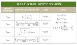
Machinedesign Com Sites Machinedesign com Files Uploads 2017 03 30 0517 Md Motor Sizing Acceleration Profiles

For the moment if we assume a maximum velocity constraint (v_lim) of 1.5m/sec then a new set of motion parameters needs to be determined using the general S-Curve solution shown in Table 2. The general S-Curve solution defines four new variables: t_cv, which is the constant velocity time; d, the constant velocity parameter; t_s1, the S-Curve acceleration time; and g, the S-Curve acceleration parameter.

Using the maximum velocity constraint (v_lim) of 1.5m/sec, total move distance (s_t) of 1.0 meter, and total move time (t_m) of 1.0 second, the constant velocity parameter is calculated to be d = 0.333, which is the solution for a 1/3 trapezoidal motion profile. The 1/3 trapezoidal motion profile has 1/3 the time in a period of constant acceleration to a maximum velocity followed by 1/3 the time in constant velocity, then 1/3 the time in a period of constant deceleration back to zero. For the 1/3 trapezoidal motion profile with full S-Curve, the S-curve acceleration parameter will be g = 0.167. The following is a list of motion profiles along with the constant velocity parameter and the S-curve acceleration parameter:

Triangular profile with no S-Curve: d = 0, g = 0

Triangular profile with 50% S-Curve: d = 0, g = 0.167

Triangular profile with full S-Curve: d = 0, g = 0.250

1/3 Trapezoidal profile with no S-Curve: d = 0.333, g = 0

1/3 Trapezoidal profile with 50% S-Curve: d = 0.333, g = 0.111

1/3 Trapezoidal profile with full S-Curve: d = 0.333, g = 0.167

Machinedesign Com Sites Machinedesign com Files Uploads 2017 03 30 Linear Motor Tecnotion Um Series Ironcore

Machinedesign Com Sites Machinedesign com Files Uploads 2017 03 30 Linear Motor Tecnotion Uc Series Ironless

For Ironcore linear motors (top), friction force applies if using mechanical bearings with a linear friction coefficient and a linear motor with attraction forces. For Ironless linear motors (bottom), there are no attractive forces between primary and secondary parts due to lack of iron in the construction. As a result, they do not experience cogging and they can travel with nearly zero force and velocity ripple. (Images courtesy of DirectIndustry.com)

The next step in sizing a linear motor with S-Curves is to calculate the RMS and peak forces using the S-Curve motion parameters and the total mass which is a combination of a preliminary linear motor coil mass (m_c) plus any payload (m_p). The peak force is the addition of the peak acceleration force (F_a) plus the peak constant forces (F_c) acting of the system such as gravity (F_g), friction (F_fr), and other external push/pull forces (F_e). The gravity force applies only if the system is tilted at angle (q) from the horizontal. The friction force applies if using mechanical bearings with a linear friction coefficient (m) and a linear motor with attraction forces (F_at) such as Ironcore linear motors. If the linear bearings have seals, the seal force (F_s) will also increase the friction force. The following formulas are used to calculate the peak force (1.2):

Machinedesign Com Sites Machinedesign com Files Uploads 2017 03 30 Equations B

With the S-Curve motion profile, the RMS or root mean square force is calculated knowing the force for both the total move time (t_m) and the dwell time (d_w). Since the S-Curve acceleration is not constant but a ramp for the acceleration and deceleration phases it can be difficult to calculate the RMS force for each specific phase of motion (acceleration, constant velocity, deceleration, and dwell). Instead, the RMS acceleration (a_RMS) will be used to calculate the acceleration force during the total move time (t_m). The follow formulas can be used to calculate the RMS force (1.3):

Machinedesign Com Sites Machinedesign com Files Uploads 2017 03 30 Equation C

Machinedesign Com Sites Machinedesign com Files Uploads 2017 03 30 Equatios D

The constant forces (F_c) apply to the total move time (t_m) and the dwell time (d_w) only if the system is tilted at angle (q) from the horizontal, and the friction (F_fr) and external push/pull forces (F_e) are greater than zero.

Machinedesign Com Sites Machinedesign com Files Uploads 2017 03 30 0517 Motor Sizing Table1

Assuming an air bearing stage with 10kg payload, zero constant forces, a preliminary coil mass of 0.5 kg, and a 2.0m/sec peak velocity, the RMS and peak forces are calculated to be 43.4N and 84.0N, respectively. Knowing these initial calculated forces, a linear motor is selected that has a continuous force (F_RMS) of 113N, peak force (F_peak) of 400N, and motor constant (K_m) of 10.2 . Using formula 1.1 the continuous power dissipated (P_RMS) is calculated to be 18.1 Watts, which multiplied by the linear motor thermal resistance (R_th) provides the motor temperature rise (DT) due to the continuous applied force. The motor thermal resistance (R_th) is listed by the manufacturer as 0.87 °C/W and the motor temperature rise (DT) is calculated to be 15.7°C.

The linear motor temperature rise (DT) should be less than the value specified by the manufacturer or the value required to achieve the desired machine accuracy. If we compare the values for the standard triangular motion profile the RMS force is 37.6N, peak force is 42N (0.5X) the continuous power dissipated is 13.6 Watts (−33%) and the motor temperature rise is 11.8°C (−3.9°C).

Machinedesign Com Sites Machinedesign com Files Uploads 2017 03 30 0517 Motor Sizing Table2

The S-curve motion profile is required for most high performance linear motor applications because it reduces impacts into the motion system and increases smoothness of point-to-point motion. However, the designer must carefully consider the S-Curve requirements during the design phase to avoid having to increase the total move time later in the build or testing phases.