By Paul Kurowski
President, ACOM Consulting, London, Ontario, Canada, Barna Szabo
Professor of Mechanics, Washington University, St. Louis, Mo.
It's easy to construct finite-element models with errors. And it's just as easy to correct them, when you know how.
The first step in a finite-element analysis selects a mathematical model to represent the object being analyzed. The term mathematical model refers to a theory such as the theory of elasticity, the Reissner theory of plates, or deformation theory of plasticity, and to the information that defines the problem - geometric descriptions, material properties, as well as constraints and loading.
The analysis goal is to compute information from the exact solution u_EX and then calculate information from it such as the maximum von Mises stress, which could be F(u_EX). The function F(u_EX) depends only on the definition of the mathematical model and not on the method used for finding an approximate solution. Therefore, it does not depend on mesh quality, type, and size of elements. The difference between F(u_EX) and the physical property it represents is called the "modeling error".
The next step uses the finite-element method to find an approximation u_FE of the exact solution u_EX. This involves selecting a mesh and elements such as 2D plates, eight-node bricks, p-elements, and so on. The mesh and elements define what’s called the finite-element discretization.
Discretization error is defined by
Most analysts would like to hold this value to no more than 10%. But modeling and discretization introduce errors. Proper application of the art and science of FEA involves assessing and controlling these two types of errors. It's also a good idea to distinguish between apparent and real errors in FEA results. By definition:
The apparent error can be less than the sum of modeling error and discretization error. The two errors can have opposite signs and may nearly cancel. The quality of results depends both on how well the model represents reality (the size of the modeling error) and how accurately the FEA software handles the transformations (the size of the discretization error).
•Engineering Software Research and Development, Inc.•
Linear Analysis: von Mises Stress
What is modeling error?
Suppose one wishes to analyze a support bracket. Questions that come to mind include: What do we want to find? Maximum stress? Maximum deflections? The first few natural frequencies? The bending stiffness? Temperature distribution? Does the bracket remain in the elastic range? How many loading conditions are critical? How should we represent support conditions?
With a clear objective and an understanding of the limitations inherent in the theory being used, analysts can create the model geometry. At times this geometry may be similar to the CAD geometry, but quite often we find it necessary to modify the topological description to simplify meshing. Part of the modeling process includes making decisions such as modeling thin walls with shell elements, taking advantage of symmetry or asymmetry or both, including or neglecting fillets, and deleting nonessential features. For example, deciding to use shell elements rather than solid elements means one makes an important decision concerning the mathematical model and hence the kind of operations the FEA software will perform.
After idealizing the topological description, one still needs to idealize material properties (select linear elastic, elastic-plastic, or another), loads, and supports. These decisions further define the mathematical problem, which supposedly represents the bracket with respect to the data of interest.
Important modeling decisions are sometimes made without much concern for their implications. It often happens that the formulated model is conceptually wrong. An indicator of a poor model comes when the strain energy corresponding to the exact solution is infinite or trivially zero. Another indicator is when the data of interest, corresponding to the solution of the mathematical model, is not defined. Or, when the solution is defined, it's entirely discretization (mesh) dependent.
Many analysts think that an efficient mesh generator reduces modeling error with a high quality mesh. It does not. Modeling assumptions are made before meshing. Consequently, even the best mesh cannot fix an improperly defined mathematical model.
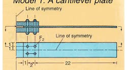
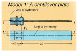
Four bolts fasten the cantilever plate. The material is ASTM A36 steel, E = 293
106 psi, Poisson's ratio = 0.295, yield stress Sy = 36.03103 psi. Assume plane stress conditions. The plate is 0.2-in. thick and fasteners are 0.4-in. diameter. Uniformly distributed traction of 1.5 3 104 psi is applied on the right edge.
A systematic approach
The only way to ensure small modeling errors is by showing that the data of interest are not sensitive to restrictive modeling assumptions. This is analogous to ensuring the discretization errors are small by showing that the data of interest are not sensitive to discretization (results do not significantly change with finer mesh or greater p value). For example, when one is interested in shearing forces along the edge of a simply supported plate, the classical plate model (Kirchhoff's plate) is unreliable. The unreliability is easily detected by using a Reissner model or a full 3D model of elasticity. A Reissner model of a plate in bending assumes that all in-plane displacements vary linearly across the thickness and that shear strains are constant across the thickness. Using higher plate models forces one to think about the meaning of a simple support, and whether or not it provides an accurate description of a physical system.
To control modeling errors in a systematic way, one needs a hierarchic point of view. A well-defined mathematical model should be viewed as a special case of a more general mathematical model. For example, a model based on the linear theory of elasticity is a special case of a model that accounts for geometric or material nonlinearities, or both. Similarly, the Reissner theory of plates is a special case of the full 3D representation, with infinitely many possible plate models in-between. When the maximum von Mises stress turns out to be larger than the yield point of the material, then a model based on the linear theory of elasticity is inappropriate. Consider a higher model, one that uses a more complex theory to imitate the real world. In any case, the linear model should be viewed only as the first step in solving a nonlinear one.
It has been difficult to control modeling errors in practice, with hierarchic models because most FEA codes link the element definition and underlying theory. For example, element libraries may describe an element as "20-node, triquadratic displacement, trilinear temperature, hybrid, linear pressure, reduced integration." Changing the model involves changing the element, which increases the complexity of the task. Modeling errors are not even considered in most cases because of the usual tight time constraints on analysis and a high level of expertise needed for properly executing the necessary computations.
A systematic approach to controlling modeling errors lags behind other FEA developments. It has been put in commercial FEA software only recently in a code called StressCheck from ESRD, St. Louis. It automatically assesses both modeling and discretization errors. The package separately handles the topological description of elements, their polynomial degree, and the underlying theory. For instance, a hierarchic family of models is available for isotropic and laminated plates in bending. The lowest member of the hierarchy is the Reissner model, the highest is a 3D representation. By repeating calculations using progressively higher hierarchic models, one can gradually "relax" modeling assumptions until the results no longer change significantly.
Modeling errors from convergence tests
Convergence analysis calculates discretization errors by increasing the number of degrees of freedom (dof) in the model by refining the mesh in h-codes or increasing element orders in p-codes. In fact, any FEA result should be produced by a convergence process rather than by a single solution. This understanding is more practical with programs based on p-element technology that makes convergence testing a part of every solution, such as Pro/Mechanica, StressCheck, and other p-codes.
A convergence test may also work as a spotter for particular modeling errors called singularities which may be masked by the discretization error. However, singularities start showing up when one examines how data of interest change after increasing the number of degrees of freedom. When data of interest do not appear to approach limiting values, then either the discretization is still too large (too few elements or too low p-order) or the model is not defined properly, or both.
Numerical convergence tests, however, do not always detect singularities and cannot be considered a foolproof singularity spotter. Should the data of interest diverge slowly, it may be difficult or impossible to detect by numerical means. The situation is analogous to computing the sum:
Hazards of Comparisons
Correlation with experiments provides an obvious and useful way to verify a wide range of modeling assumptions, and may help detect various modeling errors including singularities. But good correlation can be misleading and does not necessarily prove that the model is correct. Why? Because FEA results combine effects of two errors: the modeling and discretization error, which may nearly cancel each other, producing seemingly correct results. Suppose one wants to find the deflection of a beam supported at two points representing small rollers. A conceptual error arises by using point supports to represent rollers when the model is based on the theory of elasticity. Deflections under point support are infinite, so the FE model with many DOF will overestimate deflection.
At the same time, a coarse mesh produces a large discretization error masking the conceptual error by underestimating deflections. A credible result may be produced in that the deflection will be almost as if a roller support were properly modeled. By chance, deflections reported by the model may be quite close to what one would see in a test.
But two mistakes do not make it right. Such models are unreliable for computing stresses and reactions. Manipulating the mesh so the computed data match experimental observations is a widely practiced but bad idea. To properly evaluate and interpret results of an experiment, the errors of discretization must be smaller than the errors in experimental observations and the magnitude of discretization errors must be verified independently by the experiment.
A brief check list of modeling errors
To ensure the data of interest are accurate, ask yourself these questions about your model:
- Is the model properly conceived with respect to the data of interest?
- Is the strain energy of the exact solution finite and not zero?
- Are the data of interest finite?
- Is the estimated relative error in energy norm (not the strain energy) reasonably small, about 5% or less?
- Are the data of interest converging to a limit as the number of degrees of freedom increases?
- When stress maximums are of interest, are the stress contours smooth in the highly stressed areas?
When answers to these questions are affirmative, one can be reasonably certain that modeling and discretization errors are small. Of course, it is still necessary to test for sensitivity to modeling decisions, that is, by relaxing the assumptions as demonstrated in the examples.
How to 'relax' a finite-element model
Several finite-element models show how easy it is to make bad modeling decisions and how to control modeling errors using a systematic approach. To simplify convergence-error analysis, the models are run in p-element FEA software.
Consider a cantilever plate of a constant thickness supported by four bolts. The right edge is loaded with a normal pressure. Find the distribution of von Mises stress in the plate.
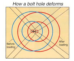
To model the cantilevered plate, an engineer might argue that the bolt diameter is small in relation to the plate, so bolts-as-point supports is a reasonable simplification. Models based on these assumptions will provide results from a single run which may seem correct because large discretization errors mask the modeling error (point supports). Any finite-element solution corresponding to a particular mesh and polynomial degree of element will report a finite stresses. However, the sketch How a bolt hole deforms shows that refining the h-element mesh or increasing the polynomial order of the p-elements around the bolts reveals increasingly large strains concentrated around the point constraints.The sketch indicates a deformed shape in the cantilever plate at bolt F2 magnified 100 times. Bolts are modeled with point constrains and the p-element order reaches eight. The underformed hole appears under the deformed shape.
How to 'relax' a finite-element model: Part 2
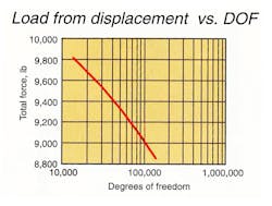
The graph Displacement versus DOF shows that in the limit (increasing DOF), the strains will be infinite on an area of zero size. Hence, the displacement of the loaded edge will be infinite.
Had one applied a prescribed displacement instead of the normal pressure to the right edge, reactions at the bolts would be zero at the limit as shown in Loads from displacement. The modeling error here is the use of point constrains which are incapable of generating nonzero reactions in the linear theory of elasticity. The numerically determined value of the reactions may look credible but it is completely dependent on the finite-element mesh and, therefore, unreliable. Running just one solution would not reveal the cardinal modeling error because it is masked by the discretization error. The point of the exercise is that convergence analysis is also a useful tool for spotting modeling errors, in this case the point supports.
A second model of the cantilevered plate tries to alleviate the problem of point supports by using linearly distributed springs for bolts around the four bolt holes. The spring rate of 3.0 3 108 lb/in. represents the elasticity of bolts. The material behavior is linear and the circular mesh around each hole has an 0.8-in. diameter.
Analysis of the cantilever plate is performed by the p-element software StressCheck. The graph indicates no convergence in maximum displacement with an increase in degrees of freedom. This is one indicator that something is amiss with the model.
Another indicator of a faulty model comes by plotting the reaction forces at the bolts versus the number of DOF when the prescribed displacement is applied to the right edge of the plate. The graph indicates that reaction at the bolts converges to zero, an illogical conclusion.
How to 'relax' a finite-element model: Part 3
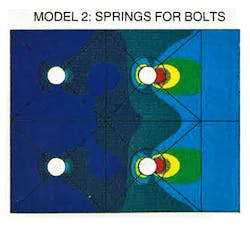
The results from Model 2: Springs for bolts shows maximum von Mises stresses of 61,600 psi. The p-code also delivers a convergence error analysis, so users can be sure the solution is sufficiently accurate. In this case, the discretization error is below 1% error in energy norm.
But how good are the reported stresses? Results show at least two problems. First, the maximum stress reads 61,600 psi while the yield stress for the plate material suggests values should not exceed 36,000 psi. For this reason, the cutoff point for the fringe plot is 36,000 psi. Because yielding has not been considered, the stress distribution shown cannot be representative of the true stress distribution, even though the error of discretization is small.
The second problem found on closer examination of stress results is that there are tensile stresses along portions of the circumference of the fastener holes. But tensile stress has no chance to develop along the plate-bolt contact area, hence the fastener-support model cannot be correct.
Both problems stem from the assumption that the cantilever plate can be modeled as a linear problem. In fact, stress above the yield point requires a model accounting for material nonlinearity while contact between bolts and plate calls for a model capable of representing mechanical contact.
| ID=SOL_LN | |
| Run=8 | |
| Fac.=Seq | |
| Max= 6.1601e+04 | |
| Min= 4.6981e+01 | |
| 3.6000e+04 | |
| 3.2002e+04 | |
| 2.8000e+04 | |
| 2.4000e+04 | |
| 2.0000e+04 | |
| 1.6000e+04 | |
| 1.2000e+04 | |
| 8.0000e+03 | |
| 4.0000e+03 | |
| 0.0000e+00 | |
bas 03
| Stress Check v2.3.b6 | 97/05/23 11:43:21 |
The distribution of von Mises stresses has been produced around the bolt holes by the linear model.
How to 'relax' a finite-element model: Part 5
For a second example, suppose one needs to find the maximum load a bracket can hold. Its material is the same as the cantilever plate. A bracket model of linear elements is "smooth" shaped without analytical problems such as singularities. It solves easily to a convergence error below 1% in energy norm. The illustration Von Mises stresses for a linear analysis shows a load of 20,000 lb producing the maximum von Mises stress of 25,609 psi. By simply scaling the load, one finds that 28,115 lb produces the yield stress of 36,000 psi and therefore plastic yielding.
A second bracket model has been updated to account for nonlinear material behavior to see how relaxing the restrictive assumptions of a linear material changes results. Because load scaling cannot be used on a nonlinear model, one needs several solutions with increasing load until the entire bracket cross-section develops stress above the limit of plasticity. Elastic-plastic Analysis shows that a 70,000-lb load does not stress all material beyond the elastic limit, indicating the bracket can carry the weight.
So the question becomes: What’s a good estimate of the ultimate load, 28,115, or 70,000 lb? It’s clearly closer to the latter, but to be sure, one needs to improve the modeling assumptions. The elastic, perfectly plastic material should be replaced with a more realistic model along with assumptions of geometric linearity (small strains and displacements) and more realistic support conditions. Nevertheless, assuming sufficiently strong supports, 70,000 lb can be reported as a conservative estimate of the ultimate load-carrying capacity. Strain hardening will increase this figure.
The objective of both exercises is not necessarily to come up with the perfect model, but rather illustrate how to deal with modeling errors in a way that gradually relaxes restrictive simplifying modeling assumptions. Then users can examine the difference the assumptions make to the data of interest.
The hierarchical approach to controlling modeling errors can be automated in special cases like plate analysis in which a series of models are formulated with progressively less restrictive assumptions. A later article will examine hierarchical plate models.
| ID=SOL_LN | |
| Run=8 | |
| Fac.=Seq | |
| Max= 3.600e+04 | |
| Min= 1.9512e+02 | |
| 3.6000e+04 | |
| 3.2002e+04 | |
| 2.8044e+04 | |
| 2.4065e+04 | |
| 2.0087e+04 | |
| 1.6709e+04 | |
| 1.2130e+04 | |
| 8.1518e+03 | |
| 4.1735e+03 | |
| 1.9512e+02 | |
bas 03
| Stress Check v2.3.b6 | 97/05/23 11:33:48 |
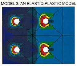
The distribution of von Mises stresses produced by the nonlinear model appears considerably different from linear model. The nonlinear solution accounts for geometric as well as material nonlinearities. The model uses springs for bolts and engages them only in compression.
| ID=SOL_LN | |
| Run=8> | |
| Fac.=Eeq | |
| Max= 3.1674e-02 | |
| Min= 6.7283e-02 | |
| 2.4828e-03 | |
| 1.2414e-03 | |
| 0.0000e+00 | |
bas 03
| Stress Check v2.3.b6 | 97/05/23 11:40:19 |
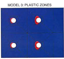
The plot shows regions where the equivalent strain exceeds the yield strain of 1.2414 3 10-3.
