How to Avoid Overengineering Composite Parts
Composites, or fiber-reinforced plastics (FRPs), give engineers a palette of options for replacing conventional low-carbon steel with lighter, more-efficient material. At the same time, these combinations of epoxy resins and carbon or glass fibers create special properties which make it difficult to calculate performance. Nevertheless, engineers can design optimal FRP parts by simulating the material’s anisotropic properties, understanding how processes affect fiber direction, and using predictive analysis.
Engineers regularly overdesign FRP parts to avoid failure, adding weight and cost that defeats the rationale for designing with new materials. Sure, the design won’t fail, but it also may not be economically competitive. A major cause of FRP overdesign is a lack of knowledge about FRP properties. There is a tendency to treat FRPs like metals with isotropic (same direction) properties instead of understanding their anisotropic (different directions) nature. In many cases, an FRP part’s anisotropic behavior can enable better performance than engineers could anticipate if they assumed “metallic” — isotropic — properties.
This file type includes high resolution graphics and schematics.
Unlike the stiffness of metal parts, which is consistent throughout their geometries, the stiffness of FRP parts can vary in different areas. That variation comes from two factors: production processes, and the alignment of carbon fibers in FRP epoxy resin matrices. The two factors are related because production processes determine the position of carbon fibers.
To illustrate this relation, assume a homogenous plastic part is subjected to a 1,000-lb load. It deflects 10 mm on its long end and 5 mm on its short end. If carbon fibers are placed along its upper surface, the FRP part deflects 3 mm on its long end and 0.25 mm on its short end. Therefore, the FRP part’s stiffness properties win over the plastic part and will perform better in crash applications.
But it can be tough to realize that stiffness because engineers need assurances that the fibers will align properly. Production process can affect the alignment. For example, the gate location on an FRP injection mold needs more design consideration than on a mold for a homogenous metal or plastic part. If a mold for the homogenous part has two gates directly opposite one another, the two material flows meet and disperse to the corners of the mold without affecting the material’s properties.
On the other hand, if two epoxy-resin flows meet in the mold, carbon fibers displace from their intended location and change alignment. To correct the problem, engineers can adjust the rate of injection or the temperature of the epoxies. But if that doesn’t work, they must change the gate positions so the flows intersect in a way that keep the fibers aligned.
To avoid trial-and-error testing, engineers need to simulate both the FRP injection-molding process and the part performance with anisotropic properties in mind. Yet, most of the FEA and simulation tools in use today treat FRPs as isotropic materials. The resulting simulation can yield less-than-accurate results.
Testing examples
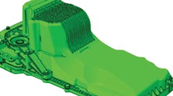
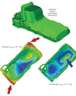
The accompanying figure labeled Isotropic versus anisotropic simulation gives proof to this theory. The red arrows indicate isotropic analysis of two potential failure points on a composite oil pan. Anisotropic analysis reveals the part does not deflect excessively at those points. An engineer relying on the isotropic analysis would likely add more mass to guard against failure which will not occur.
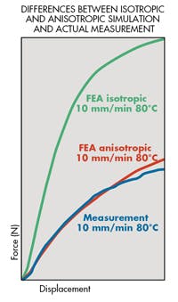
Another example of isotropic versus anisotropic simulation is visible in the chart labeled Differences between isotropic and anisotropic simulation and actual measurement. The blue line is an FEA comparison curve and represents the actual physical measurement of a composite prototype. The variance in results between the isotropic analysis and the physical measurement is more than 80%. The anisotropic analysis curve closely resembles the physical testing.
Modeling anisotropic propertiesThe energy-management company Schneider Electric in France and FRP supplier DuPont, Wilmington, Del., redesigned a bracket in FRP. The companies used predictive analysis to modify and optimize the FRP bracket design. Engineers analyzed the design in two materials to determine the breaking-point stiffness based on the fiber orientation. One of the materials was made of 20% glass-fiber-reinforced polymer and the other was 50% glass-fiber-reinforced polymer. Production-process models were then imported into a nonlinear, multiscale material and modeling platform. The designs were analyzed using isotropic and anisotropic material properties. The isotropic analysis varied 85% for the 20% material and 120% for the 50% material. The anisotropic testing produced a curve that differed from the physical measurements by only 5% for the 20% material and 2.5% for the 50% material. Clearly, the anisotropic results produced a smaller variation between simulated and actual results. This helped the companies find an optimal design. If the companies relied on the isotropic analysis alone, the variation between the simulated and actual results would be too large and unpredictable for engineers to design with the maximum possible precision. Instead, they would overdesign to avoid failure. |
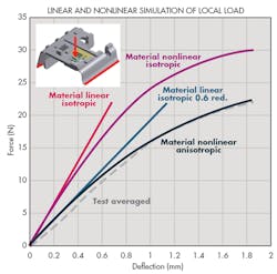
The same pattern emerges on the chart called Linear and nonlinear simulation of local load. The chart shows the testing of a sunroof bearing under a local load with the bottom sides of the part fixed. It compares the accuracy of nonlinear anisotropic simulation with linear and nonlinear isotropic simulation. The dotted line represents the averaged results from physical testing. The anisotropic, nonlinear analysis is almost identical to the physical testing. When results are close, models can go from computer to production without multiple rounds of physical prototyping. Use of computational analysis modeling and simulation methods early in the design process to predict the performance of a part is called predictive analysis.
Predictive analysis over benchmarking
Anisotropic analysis is a major component of predictive analysis. Most types of analysis software incorporate some level of anisotropic material behavior to help engineers approximate FRP behavior. For example, FRPs are represented as “black aluminum” — a kind of placeholder that accurately depicts FRP part geometry. However, this placeholder does not depict its anisotropic properties. In addition, current FEA and simulation software products benchmark the results, which is a comparative process, rather than create a predictive process.
Benchmarking takes place when engineers run an FEA analysis of a design and then make a physical part and compare it to the initial FEA. Correlations are made to the FEA model until it represents the final product behavior. The benchmark provides data for the remainder of the project and future projects. This method works for metals, but because the shape and fiber alignment in each FRP part gives varying stiffness, benchmarking can prove to be unreliable for deciding mass and geometry.
Predictive analysis can reduce time to production. However, a fast production process that yields erratic quality can be self-defeating. To use predictive analysis successfully, engineers need to understand three things: the individual properties of the fiber and the matrix, the composition of the overall materials, and how manufacturing processes influence them.
The three elements can be understood with the help of FEA and simulation tools. Specific tools that are helpful include smart material data models and fiber orientation maps. “Smart” in this context means employing material data sets that, given any fiber alignment, can tell you the exact stress-frame response. The fiber orientation information comes from process simulation software that depicts the group of fibers in the epoxy resin matrix that emerges from the production process.
These tools let engineers see the stress frame response for each section of the design. They can use that knowledge to reduce mass where possible and increase it where needed.
Edited by Lindsey Frick, [email protected], @MaterialShout
Resources: Digimat Software, http://www.e-xstream.com/en/digimat-software/;
http://www.e-xstream.com/event.html/DIGIMATUM09/Proceedings/digimatum09_ticona_why_anisotropic_simulations_are_necessary.pdf
This file type includes high resolution graphics and schematics.


